CPU Scheduling क्या है? Algorithms, Types और Examples हिंदी में

CPU Scheduling क्या है? — Algorithms, Types और Examples

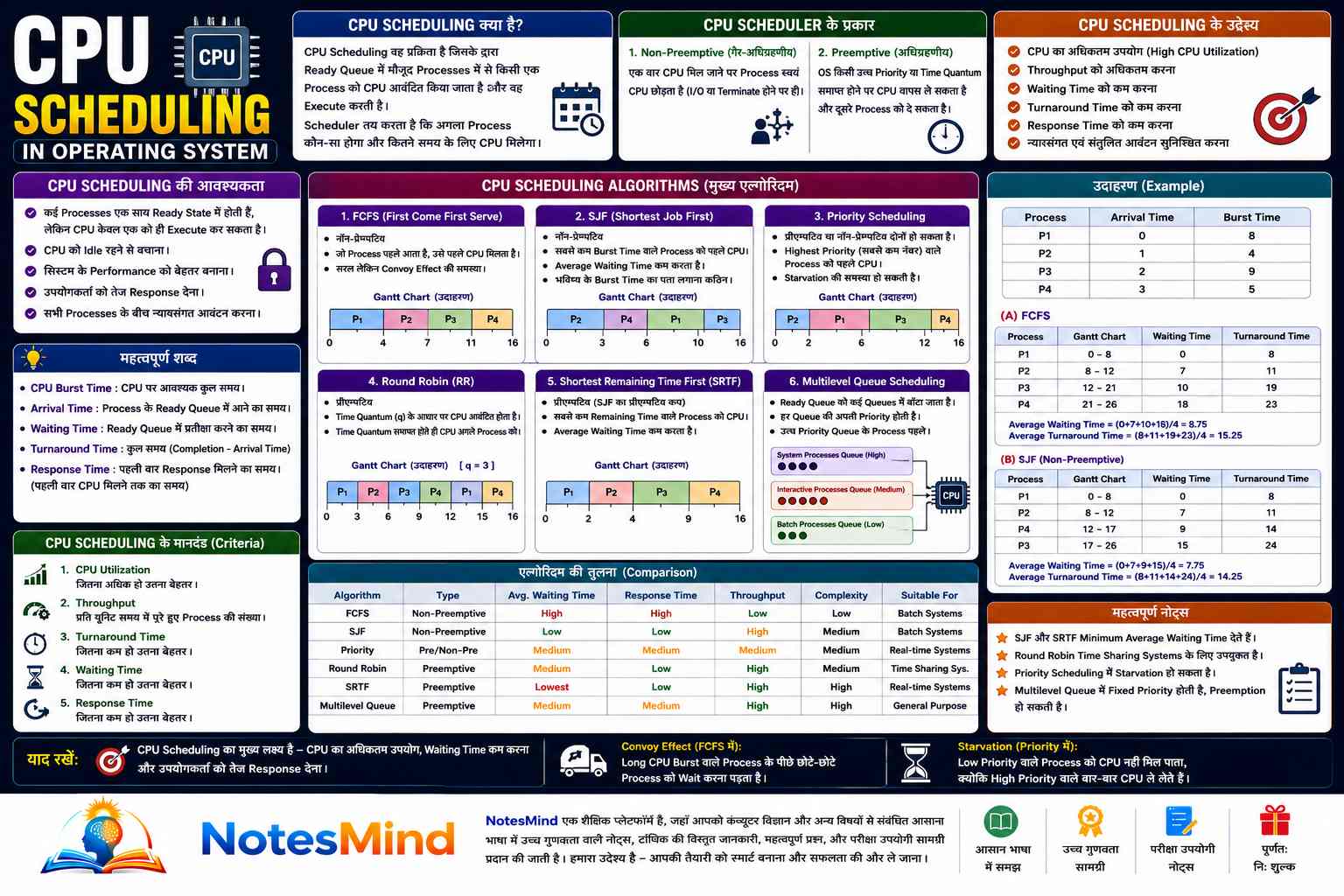
CPU Scheduling वह process है जिसमें Operating System यह decide करता है कि Ready Queue में मौजूद processes में से कौन सा process अगला CPU पाएगा।

जब एक साथ कई programs चल रहे हों और CPU एक ही हो — तो किसे पहले chance मिलेगा? यह decision CPU Scheduler लेता है। इसके बिना CPU idle पड़ा रहेगा, programs slow होंगे, और users को lag महसूस होगा।

CPU Scheduling is the process of selecting one process from the Ready Queue and allocating the CPU to it.

Turnaround Time और Waiting Time को minimize करना, और CPU Utilization को maximum रखना — यही CPU Scheduling का असली goal है।

---

Real Life Example — Bank Counter

एक bank में एक Cash Counter है, लेकिन 10 customers लाइन में हैं। अब Bank Manager decide करेगा — किसे पहले serve करें?

Customers    →  Processes
Cash Counter →  CPU
Bank Manager →  Operating System

यही काम Computer में CPU Scheduler करता है — बस customers की जगह processes होती हैं।

---

CPU Scheduling क्यों ज़रूरी है?

Scheduling न हो तो:

Problem	Effect
CPU Idle रहेगा	Processing time waste
Programs slow होंगे	User experience खराब
Response Time बढ़ेगी	Interactive systems fail
Throughput कम होगा	कम काम, ज़्यादा time
Resources waste होंगे	Inefficient system

इसीलिए OS हमेशा CPU को busy रखने की कोशिश करता है।

---

CPU Scheduling के 6 मुख्य Objectives

1. Maximum CPU Utilization

Without Scheduling: CPU ──── Idle ────
With Scheduling:    P1 → P2 → P3 → P4

2. Maximum Throughput

 

 

1 Minute में:
Without Scheduling → 3 Processes complete
With Scheduling    → 8 Processes complete

3. Minimum Waiting Time

Ready Queue में process को कम से कम इंतज़ार करना पड़े।

4. Minimum Turnaround Time

Turnaround Time = Completion Time − Arrival Time

5. Minimum Response Time

पहली बार CPU मिलने में कम time लगे। Interactive systems में यह सबसे important है।

6. Fairness

हर process को CPU मिले — कोई भी हमेशा wait में न रहे।

---

CPU Scheduler कैसे काम करता है?

Ready Queue
  P1, P2, P3, P4
        │
        ▼
   CPU Scheduler
        │
        ▼
       CPU

OS का वह part जो Ready Queue से process चुनता है — वही CPU Scheduler है।

---

तीन Types के Schedulers

Schedulers
  ├── Long Term Scheduler
  ├── Medium Term Scheduler
  └── Short Term Scheduler

1. Long Term Scheduler (Job Scheduler)

New jobs को disk से उठाकर Ready Queue में लाता है। Degree of Multiprogramming control करता है — यानी एक समय में कितने processes memory में रहेंगे।

 

 

Disk → Long Term Scheduler → Ready Queue

2. Short Term Scheduler (CPU Scheduler)

Ready Queue से अगला process select करता है। यह सबसे ज़्यादा बार execute होता है — milliseconds में।

 

 

Ready Queue → CPU Scheduler → CPU

3. Medium Term Scheduler

Swapping करता है — process को memory से disk पर भेजना और वापस लाना।

Main Memory → Swap Out → Disk → Swap In → Memory

Scheduler	काम	Frequency
Long Term	Jobs को memory में लाना	Infrequent
Short Term	CPU allocate करना	Very frequent
Medium Term	Swapping	Occasional

---

Preemptive vs Non-Preemptive Scheduling

Non-Preemptive Scheduling

CPU मिलने के बाद process खुद complete होती है — बीच में कोई CPU नहीं छीन सकता।

 

 

P1 ──────────── Finish
P2              Wait...
P3              Wait...

Examples: FCFS, Non-Preemptive SJF, Non-Preemptive Priority

Preemptive Scheduling

OS ज़रूरत पड़ने पर process से CPU वापस ले सकता है।

P1 runs → Time Over → CPU वापस → P2 runs

Examples: Round Robin, SRTF, Preemptive Priority

Feature	Non-Preemptive	Preemptive
CPU छीना जा सकता है?	❌	✅
Response Time	ज़्यादा	कम
Context Switching	कम	ज़्यादा
Interactive Systems	खराब	अच्छा

---

CPU Scheduling Algorithms — विस्तार से

---

1. FCFS — First Come First Serve

Definition: जो process पहले arrive करे, उसे CPU पहले मिले। Ticket counter की तरह — पहले आओ, पहले पाओ।

Example:

Process	Arrival Time	Burst Time
P0	0	5
P1	1	3
P2	2	8
P3	3	6

Gantt Chart:

0        5        8        16       22
|   P0   |   P1   |   P2   |   P3   |

Waiting Time Calculation:

Waiting Time = Service Time − Arrival Time

Process	Service Time	Arrival Time	Waiting Time
P0	0	0	0
P1	5	1	4
P2	8	2	6
P3	16	3	13

 

 

Average Waiting Time = (0 + 4 + 6 + 13) / 4 = 5.75 ms

फायदे ✅	नुकसान ❌
सबसे आसान algorithm	Convoy Effect होता है
कम overhead	Average waiting time ज़्यादा
Implement करना simple	Interactive systems के लिए poor

Convoy Effect क्या है? एक long process सबके आगे आ जाए तो सब छोटी processes उसका इंतज़ार करती रहती हैं — जैसे highway पर एक slow truck सबको रोक दे।

---

2. SJF — Shortest Job First

Definition: जिस process का Burst Time सबसे कम हो, उसे पहले CPU मिले।

Example:

Process	Burst Time
P0	5
P1	3
P2	8
P3	6

Execution Order: P1 (3) → P0 (5) → P3 (6) → P2 (8)

Gantt Chart:

0      3      8      14      22
|  P1  |  P0  |  P3  |  P2  |

Waiting Time:

Process	Waiting Time
P1	0
P0	3
P3	8
P2	14

Average Waiting Time = (0 + 3 + 8 + 14) / 4 = 5 ms

फायदे ✅	नुकसान ❌
Minimum average waiting time	Burst time पहले से पता होना चाहिए
Best theoretical performance	Starvation हो सकता है

Burst time predict करना practically मुश्किल है — यही SJF की सबसे बड़ी limitation है।

---

3. Priority Scheduling

Definition: हर process को एक priority value मिलती है। Highest priority वाला process पहले execute होता है।

Example:

Process	Priority
P0	1
P1	2
P2	1
P3	3

अगर 1 = Highest Priority, तो execution order:

P0 → P2 → P1 → P3

समान priority होने पर FCFS apply होता है।

फायदे ✅	नुकसान ❌
Important jobs पहले complete	Low priority process starve हो सकती है
Real-time systems के लिए useful	Aging implement करना पड़ता है

Solution — Aging: जितना ज़्यादा wait करो, priority उतनी बढ़ती जाए — eventually CPU ज़रूर मिलेगा।

---

4. Round Robin Scheduling

Definition: हर process को एक fixed time (Time Quantum / Time Slice) मिलता है। Time खत्म हुआ — CPU वापस, अगली process की बारी।

यह Preemptive algorithm है। Interactive systems के लिए सबसे suitable।

Example (Time Quantum = 3 ms):

Process	Arrival Time	Burst Time
P0	0	5
P1	1	3
P2	2	8
P3	3	6

Execution:

0-3:  P0 (3 ms)
3-6:  P1 (3 ms) → P1 Complete ✅
6-9:  P2 (3 ms)
9-12: P3 (3 ms)
12-14: P0 (2 ms) → P0 Complete ✅
14-17: P2 (3 ms)
17-20: P3 (3 ms) → P3 Complete ✅
20-22: P2 (2 ms) → P2 Complete ✅

Gantt Chart:

0   3   6   9  12  14  17  20  22
|P0 |P1 |P2 |P3 |P0 |P2 |P3 |P2 |

फायदे ✅	नुकसान ❌
Fair scheduling	Context switching ज़्यादा
Interactive systems के लिए best	Time quantum बहुत छोटा हो तो performance गिरती है
Response time अच्छा	Time quantum बड़ा हो तो FCFS जैसा हो जाता है

Time Quantum कितना होना चाहिए? न बहुत छोटा, न बहुत बड़ा। Practically 10-100 ms standard माना जाता है।

---

5. Multi-Level Queue Scheduling

अलग-अलग type की processes को अलग-अलग queues में रखा जाता है — हर queue का अपना algorithm होता है।

Highest Priority
      │
      ▼
System Processes Queue      → Priority Scheduling
      ▼
Interactive Queue           → Round Robin
      ▼
Editing Queue               → Round Robin
      ▼
Batch Queue                 → FCFS
      ▼
User Queue                  → FCFS
      │
Lowest Priority

Queue	Scheduling Algorithm
System	Priority
Interactive	Round Robin
Batch	FCFS

Real systems जैसे Linux और Windows इसी concept का use करते हैं — different processes को different treatment मिलती है।

---

सभी Algorithms की तुलना

Algorithm	Preemptive	आधार	फायदा	नुकसान
FCFS	❌	Arrival Time	सबसे simple	Convoy Effect, high wait time
SJF	❌ (SRTF = ✅)	Shortest Burst	Minimum waiting time	Burst time predict करना मुश्किल
Priority	दोनों	Priority Value	Important process पहले	Starvation
Round Robin	✅	Time Quantum	Fair, best for interactive	ज़्यादा context switching
Multi Queue	दोनों	Multiple Queues	Different processes के लिए flexible	Complex management

---

FAQ — CPU Scheduling के Common Questions

Q1. Round Robin में Time Quantum कितना बड़ा होना चाहिए?

Time Quantum बहुत छोटा हो तो context switching overhead बढ़ता है — CPU time process switch करने में waste होती है। बहुत बड़ा हो तो Round Robin basically FCFS बन जाता है। Practically 10ms से 100ms के बीच रखा जाता है। Rule of thumb — Time Quantum, average burst time से थोड़ा ज़्यादा होना चाहिए।

Q2. SJF को Optimal क्यों कहते हैं लेकिन practically कम use होता है?

SJF theoretically minimum average waiting time देता है — इसीलिए optimal है। लेकिन practically, OS को पहले से नहीं पता कि अगले process का burst time कितना होगा। इसे predict करना पड़ता है — और prediction हमेशा accurate नहीं होती। यही practical limitation है।

Q3. Preemptive और Non-Preemptive में कौन सा better है?

यह situation पर depend करता है। Interactive systems (web browsers, games, ATM) में Preemptive better है — response time कम रहता है। Batch processing (video rendering, data backup) में Non-Preemptive ठीक है — context switching overhead कम होता है। Modern OS दोनों mix करते हैं।